
I mentioned in a previous post on how to get (nearly) live stock data from Google Finance. However, if you start pulling data from different markets, daily historical rates won’t make sense as different markets are closed on different days. This causes problems when trying to figure out the correlation between stocks. A solution to this is to pull monthly rates as the adjusted stock price for each month will be a better indicator of correlation.
Python has a great library called pandas_datareader that allows you to pull in historical information right into a pandas dataframe. The only downside is if an API is deprecated, your code breaks. Hence, I’ve elected to create this tutorial using Yahoo Finance’s Historical data download function. The objective of this article is to pull a large amount of worldwide historical data (over 20 years worth) and then use Modern Portfolio Theory (Mean Variance Optimization) to create an efficient frontier. The efficient frontier can help decide asset allocations in your portfolio based on a given risk tolerance and expected return.
Overview
The goal of the portfolio optimization is to retrieve an annualized expected return for a given risk tolerance. The return is associated with a portfolio of weightages (asset-allocation) to help decide investment strategies. The optimization strategy that will be used in this analysis is Modern Portfolio Theory (Markowitz, 1952), commonly known as Mean Variance Optimization (MVO) introduced by Harry Markowitz in 1952. The MVO model only takes into consideration historical results and thus is limited to that. It will not be able to account for other factors that could affect a model such as ‘views’ or insight into future market forecasts. A more robust model that could be incorporated in future optimizations is the Black-Litterman Model (Black & Litterman, 1992) that enhances the asset-allocation process by introducing user input for specific opinions on market returns.
Data Collection
Throughout this post, I will guide you through an excel workbook so you can understand exactly what is happening. If you’d like, you can download the excel workbook here.
In order to avoid high active management costs, I’ve elected to use Index Funds as the selected assets for the optimization. Market indices have the longest history of stock information and won’t have the risks of individual company stocks. Historically markets have grown and by using market indices, the expected return will be at the market average, which is far better than trying to outperform the market year after year. In addition, indices helped provide greater exposure, both in terms of geographic location and in terms of type of asset. The following indices were chosen for the optimization (Table 1).
| Index | Name | Country | Type |
| ^DJI | Dow Jones Industrial Exchange | US | Equity |
| ^IXIC | Nasdaq | US | Equity |
| GSPTSE | Toronto Stock Exchange | Canada | Equity |
| N225 | Nikkei 225 | International | Equity |
| GSPC | S&P500 | US | Equity |
| XOI | NYSE Arca Oil Index | Worldwide | Commodity |
| HUI | HUI Gold Index | Worldwide | Commodity |
| HIS | Hong Kong Stock Exchange | International | Equity |
| FBIDX | Fidelity® U.S. Bond Index Fund Investor Class | US | Fixed Income |
| VEIEX | Vanguard Emerging Mkts Stock Idx Inv | International | Equity |
| FBNDX | Fidelity Investment Grade Bond | US | Fixed Income |
| TYX | Treasury Yield 30 Years | US | Fixed Income |
| VBMFX | Vanguard Total Bond Market Index Inv | US | Fixed Income |
| VEURX | Vanguard European Stock Index Investor | Europe | Equity |
Table 1. Breakdown of assets chosen for optimization
Since the investors will be Canadians, I look at the geographic outlook in three different areas: Canada, the US, and International. Also, by type of assets, a mixture of equity, fixed income, and commodities were chosen.
Since the optimization would look at upwards of 30 years in the future, the more data collected, the better. Data was collected from July 1st, 1996 to March 1st, 2018 to account for approximately 22 years of data. It was a trade-off to either get more years of data or exclude the fixed income funds due to the limited data available for those assets. To avoid inconsistent dates for data collection due to different market closures worldwide, monthly data was collected. This time frame covers a few market crashes including the Asian Financial Crisis (Michael & John, n.d.) in 1997, the Dotcom Crash (Beattie, Market Crashes: The Dotcom Crash (2000-2002), n.d.) from 2000-2002, and the Housing Bubble/Credit Crisis (Beattie, Market Crashes: Housing Bubble and Credit Crisis (2007-2009), n.d.) of 2007-2009.
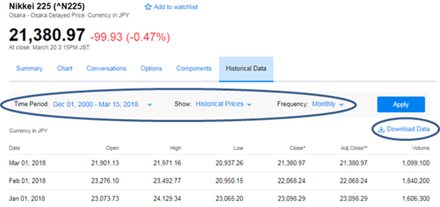
Adjusted monthly close price was pulled from Yahoo Finance (Historical Stock Data) by applying filters to pull from the following parameters:
- Time Period: Jul 01, 1996 – Mar 1, 2018
- Show: Historical Prices
- Frequency: Monthly
Data for each asset was collected in that indices’ respective currency and outputted to a csv file. Currency conversion was not required as the percentage return was calculated for returns.
Optimization Process
Monthly Returns
The adjusted closing prices were taken from each index and then collated into a table.
After that the monthly returns were calculated as a percentage by subtracting the closing price of a previous month form the closing price of the current month and then dividing that by the closing price of the previous month.
Ri = (ClosingPricei – Closing Pricei-1) / Closing Pricei-1
An average of the all the returns was taken to get the average monthly return for each asset. Then those averages were multiplied by 12 to get an annualized average return.
Covariance and Standard Deviation
A covariance matrix was created by comparing each asset with all the other respective assets. This matrix is essential in understanding the risk of each asset and how it relates to the others.
The standard deviation for each asset was taken by looking at the monthly returns. This was then used to calculate the correlation matrix.
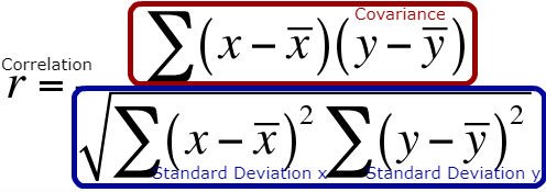
The top part of this formula is the Covariance matrix in the excel workbook and the bottom part is the D Matrix. By dividing these two, you get the Correlation Matrix.
Correlation
Correlation is important in understand how similar two assets are. The higher the correlation, the more likely they are to move in the same direction. Negative correlation implies that if one asset goes up, the other will go down and vice versa.
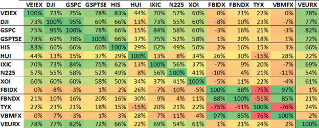
As expected, assets have 100% correlation with themselves. In addition, the S&P500 (GSPC) is 95% correlated with the Dow Jones Industrial Exchange (DJI). This is intuitive as there is a lot of overlap between the two indices. Another interesting finding is that Treasury Bills are heavily negatively correlated with corporate bond indices.
Efficient Frontier

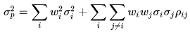
In order to create an efficient frontier, the expected return E(Rp) was maximized while constraining the standard deviation σp to specific values. The weights of each asset i, is wi. The correlation coefficient ρij is the correlation between assets i and j.
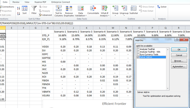
Before we do anything, it is important to remember to annualize the Expected Returns and Standard Deviations. Since we took monthly closing prices, multiple them by 12 as seen by cell A2 in this worksheet.
Excel’s Solver plugin was used to calculate these maximum points. If you don’t already have solver added in, go to File -> Options -> Add-Ins -> Manage: Excel Add-Ins Go -> Click Solver Add-in and select OK. If done correctly, you should now see the Solver option in the Data pane on excel.
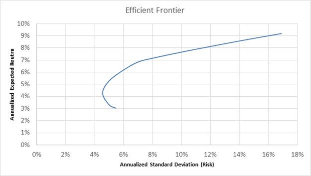
The weightage of each asset was constrained to positive values to avoid short selling and with an upper bound of 20% to ensure diversification. The solver was run for multiple different iterations of Standard Deviation for the portfolio (STD_P) to get different points for the efficient frontier. After about 15 scenarios, the Expected Return of the Portfolio (E(R_P)) was graphed against the STD_P to get your efficient frontier. To ensure you get a nice frontier, be sure you maximize the Expected Return, but also minimize it. Of course you’ll only care about the maximum expected return because why would you want less money?
As expected, portfolios with a higher return were exclusively in equities which have higher risk and portfolios with the least amount of risk were heavily weighted into the fixed-income assets.
The optimal point with minimal risk is an annual Expected Return of 4.55% and a portfolio consisting of the following assets:
| Ticker | Weightage |
| DJI | 0.11 |
| GSPTSE | 0.08 |
| HUI | 0.01 |
| N225 | 0.03 |
| FBIDX | 0.20 |
| FBNDX | 0.20 |
| TYX | 0.16 |
| VBMFX | 0.20 |
Works Cited
Beattie, A. (n.d.). Market Crashes: Housing Bubble and Credit Crisis (2007-2009). Retrieved from Investopedia: https://www.investopedia.com/features/crashes/crashes9.asp
Beattie, A. (n.d.). Market Crashes: The Dotcom Crash (2000-2002). Retrieved from Investopedia: https://www.investopedia.com/features/crashes/crashes8.asp
Black, F., & Litterman, R. (1992). Global Portfolio Optimization. Financial Analysis Journal, 28-43.
Historical Stock Data. (n.d.). Retrieved 03 16, 2017, from Yahoo Finance: https://finance.yahoo.com/quote/%5EN225/history?period1=975646800&period2=1521086400&interval=1mo&filter=history&frequency=1mo
Markowitz, H. (1952). Portfolio Selection. The Journal of Finance, 77-91.
Michael, C., & John, C. (n.d.). Asian Financial Crisis. Retrieved from Federal Reserve History: https://www.federalreservehistory.org/essays/asian_financial_crisis
Disclaimer — The material in this article is provided for informational purposes only. It is not a recommendation to buy or sell any security or implement any investment strategy.